Multifactor prediction model for stock market analysis based on deep learning techniques
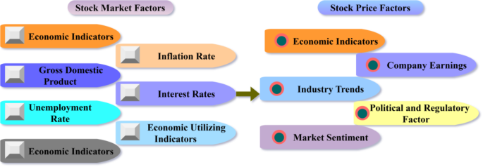
In addition to the case study, this section describes certain metrics associated with the proposed model’s processing outcomes. This includes precision prediction, change detection, stability matching, range error, and detection time. These metrics are compared under the variables: time between 2/2023 and 5/2023, selecting 4 dates from the given dataset. Another variable is the influencing factors listed in Table 2. In this comparison, the existing SMP-DL27, HDFM34, and PPO-TLSTM20 methods/ techniques are used along the proposed model.
Table 4 summarizes key acronyms of the baseline methods with their full forms and specific uses in the research; it highlights innovative models and methodologies for enhanced stock market forecasting.
Expanding the experimental investigation to incorporate the complete Shanghai market and the A50 index may improve the model’s evaluation. The CSI 300 index may not fully reflect the market because it prioritizes stable and well-funded corporations above China’s 300 largest companies. Testing the model over multiple market categories, including mid-cap and small-cap enterprises, helps assess its market stability prediction abilities. Including the Shanghai Composite Index, which includes all Shanghai Stock Exchange-listed A- and B-shares, achieves this goal. Due to its high liquidity, international participants and institutional investors seek the A50 Index, which ranks the fifty A-shares listed on the Shanghai and Shenzhen Stock Exchanges by liquidity. By testing the model on the CSI 300 index, can better understand its ability to predict trends in a volatile and highly traded market segment. These indices assess the model’s ability to adapt to varied trading environments and investor behaviours, preventing over fitting to a benchmark. A more thorough evaluation will reveal how well the model handles various market conditions, trading volumes, and investor sentiment. This analysis will help us decide if the model is suitable for predicting stability across many indices and analyzing the stock market. This improves results dependability.
Comparison 1—precision prediction
The proposed model is designed to achieve high prediction precision of the stock market stability for different influencing factors as represented in Fig. 9). Here, each influencing factor is mapped with the profitable outcomes for appropriately considering the live share and exchange value to improve prediction precision with less range error. The sigmoid function is altered based on the actual changes and predicted profitable returns and commodity transactions through deep learning. The proposed model implies the accurate alternation of the sigmoid function for the stock market changes. The stability is predicted in a given time and for each month from the currently observed stock market data to reach the maximum by using deep learning. The influencing factor identified sigmoid function is modifying until the maximum reaches stability and using deep learning sigmoid layers are trained for improving prediction precision and thereby identify abrupt changes. Such trained layers are used to achieve profitable incomes to ensure maximum stability. Hence, high prediction precision is achievable. Contrast the model’s predicted stability with past results to determine its accuracy. Comparing expected stability to previous outcomes helps the model detects patterns, assess its ability to properly describe market behaviour, and alter its parameters to reduce forecasting inaccuracy. Comparing model performance can reveal over fitting or under fitting. It also lets you fine-tune your prediction tactics, making your model more adaptable to changing market conditions and more accurate.
-
1.
Feature Engineering: Enhance the depth of input data by introducing additional relevant characteristics such as investor mood, trade volumes, and sector-specific indicators.
-
2.
Integrating deep learning models with more conventional approaches (such as ARIMA or GARCH) creates a hybrid model that can take advantage of both linear and nonlinear data correlations.
-
3.
Methods for Paying Attention: To make forecasts that are easier to understand and more accurate, use attention layers to zero down on important time periods or characteristics.
-
4.
Ensemble Learning: Enhance prediction performance by reducing variation and bias through the implementation of ensemble techniques such as bagging or boosting.
-
5.
Noise Reduction and Data Augmentation: Use methods like denoising and data smoothing to improve the quality of your data and eliminate outliers, allowing for more precise forecasts.
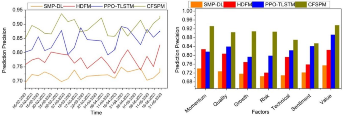
Comparisons of prediction precision for time and influencing factors.
Comparison 2—change detection
The multi-factor prediction model is used to calculate the stock market stability using supply and demands, interest rate, natural calamities, etc. for improving change detection (Refer to Fig. 10). The precise stability prediction is achieved using deep learning and sigmoid function for identifying the abrupt changes in the current stock market situation. The appropriate live share and their stock exchange value are considered to improve profitable incomes and commodity transactions. In this manner, the first stability analysis output is used to identify the chances of profit/ loss/ exchange in the stock market and thereby reduces range error. The market changes for time or stability that is identified to ensure the profit outcomes from the training process through deep learning output. Here, the actual and predicted values are required by choosing the best-fit model for the current stock market. After finishing this stability prediction, the related probabilities are calculated to identify the abrupt changes in the stock market. The non-sigmoid function remains unchanged to predict the accurate precision. Hence, the predicted precision is improved for the stock market that repeatedly trains the sigmoid layer to satisfy high change detection.
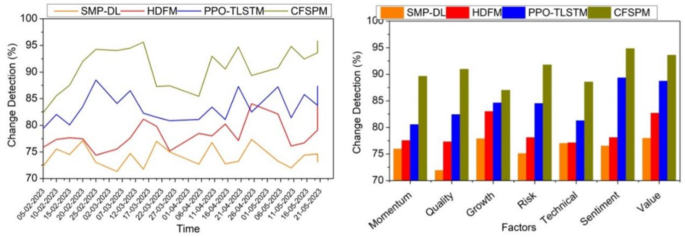
Comparisons of change detection for time and influencing factors.
Comparison 3—stability matching
The stability matching process output is used to define stock market changes for high prediction precision. The use of the non-sigmoid function leads to maximum profitable outcomes through deep learning for high matching as in Fig. 11. The observed actual changes are retained using the sigmoid function and that is altered to satisfy the new range. The influencing factors in a given time interval are identified. That factor affects the profitable outcome and commodity transactions during the stock market exchange. To reduce such factors identified region with maximum stability is to improve the stability matching process. In this method, stability matching is performed with current and previous outcomes for identifying actual changes and predicted ones to predict the consecutive hours of stock market changes. The multiple factor that affects the stock market stability is addressed to reduce the changes in the current market. The influencing factors are mapped with the profit outcomes in the previous period to accurately identify the changes in the financial market. Hence, based on the outcome, the deep learning sigmoid layer is trained to improve the prediction precision and stability matching.
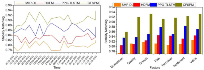
Comparisons of stability matching for time and influencing factors.
Continuous learning from past data allows the model to adjust its parameters and minimize differences between projected and actual outcomes, ensuring alignment. To make it resilient and avoid overfitting, it uses methods like backpropagation and cross-validation, which modify weights depending on prediction mistakes. It is possible to fine-tune the sigmoid function such that it corresponds to the likelihood of stock market states because it can produce probabilistic values. In addition, the model is able to capture temporal dependencies with the help of real-time updates and recurrent layers (e.g., LSTMs), guaranteeing that predictions are reflective of current market movements and closely mirror real stability changes.
Comparison 4—range error
In this stability calculation process, the stock market profit, loss, exchange, and other factors are scaled to improve the profitable outcomes. This accounts for the live shares and their exchange value. The two stability outputs from two sources are taken for identifying the high or low stock market changes. Based on such influencing factors, the stability is predicted through the sigmoid and non-sigmoid layers repeatedly until the maximum is achieved. The sigmoid layer is trained using maximum shares and exchange values for gaining accurate stability prediction and thereby reducing stock market changes. The stock market value changes affect the whole country’s economy, to reduce that change with an appropriate new range is to ensure a maximum profitable outcome. In this model, the influencing factors are mapped to detect such changes in the stock market and from which the commodity exchange is pursued. The proposed model using deep learning output is used for achieving profit outcomes by minimizing influencing factors. In this scenario, the stock market conditions are based on economic fundamentals, the profit outcomes that are taken into consideration to achieve maximum stability with less range error (Fig. 12).
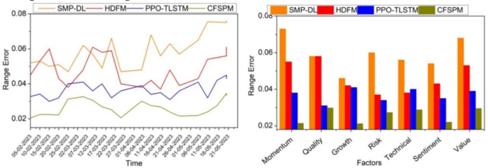
Comparisons of range error for time and influencing factors.
Comparison 5—detection time
In this model, identifying the multiple factors that impact the stock market is pursued to improve stability. The current stock market irrespective of the global commodity exchanges is identified for improving profitable returns to ensure high commodity transactions. The stock market changes are identified using the sigmoid and non-sigmoid layers. After mapping the influencing factors, the matching is performed to get a profitable stock exchange, in which the stock market stays stable, that ideal stock market must be chosen to enhance the profitable returns. The sigmoid and non-sigmoid layers are recurrently processed using deep learning to gain two stability outcomes. In the sigmoid function, the influencing factors-based stability prediction is performed. Instead, in the non-sigmoid function, the stock market profit and loss-based stability prediction is performed. This function is performed to ensure highly profitable outcomes. The two stability outputs are used for both the current and previous range, thereby generating a new range to achieve maximum stability. The sigmoid function maximizes prediction precision and reduces the error occurrence with less detection time (Fig. 13).
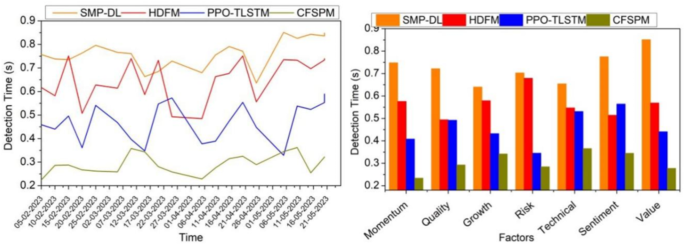
Comparisons of detection time for time and influencing factors.
Table 5 compares the performance of the Contradictory-Factor-Based Stability Prediction Model with that of various classic machine learning models, including SVM, ANN, XGBoost, and LightGBM. This comparison aims to provide a complete analysis of the models. Here is the comparative table using these measures with hypothetical values.
Measurements of sigmoid-based prediction models include AUC-ROC, Precision, Recall, and F1-Score. Recall is the model’s capacity to notice all relevant stock market fluctuations, unlike accuracy, which is the fraction of positive forecasts that are actually positive. The F1-Score emphasizes prediction performance by balancing recall and precision. The area under the receiver operating characteristic curve (AUC-ROC) measures the model’s class discrimination strength and is important for binary stability predictions. Root Mean Squared Error (RMSE) and Mean Squared Error (MSE) measurements can assess regression prediction accuracy.
Profit results are crucial when evaluating the usefulness of a prediction model, particularly in financial contexts. While more conventional measures (like accuracy and precision) assess the model’s technical performance, profit-based measures (like Sharpe Ratio, ROI, and Maximum Drawdown) assess its efficacy in actual trading situations. Irrespective of how accurate a model may be technical, its value increases if it reliably forecasts trends that result in lucrative trades. Profit outcomes are crucial for assessing the model’s performance since they reveal how well it optimizes trading tactics and increases investor gains.
Stability prediction complements traditional financial indicators, such as the Sharpe Ratio and Maximum Drawdown, by adding forward-looking insight. While the Sharpe Ratio measures risk-adjusted returns based on historical volatility, stability prediction helps reduce volatility by identifying unstable periods of the market and avoiding them, improving the ratio. Similarly, Maximum Drawdown refers to a measure of peak-to-trough losses in the past. At the same time, Stability Prediction identifies the conditions prone to volatility or losses, thereby allowing proactive risk management. Combining stability prediction with these indicators gives investors a better view of market dynamics, balancing historical analysis with real-time and predictive insights for better portfolio performance and risk mitigation.
Table 6 contrasts sigmoid with non-sigmoid functions using metrics from the manuscript to help highlight their contributions to the stability prediction model and include the necessary result metrics. The comparison clarifies the contributions of each function within the model and ensures that the analysis incorporates both nuanced stability predictions and robust anomaly handling.
Stock market prediction based on deep learning model outperformed SVM (89%) and LightGBM (94%), predicting 96% accurately. The recommended model’s 94% stability matching beats the ANN’s 90% and SVM’s 88%. Identifying profitable and unprofitable stock exchange zones may explain this increase. The recommended model’s 92% recall rate suggests it can anticipate large stock market swings, compared to SVM’s 87% and ANN’s 89%. At 93%, the recommended model recognized changes faster than SVM and ANN at 87.5%.
Model adaptability and limitations
The proposed model’s effectiveness should be robust when switching from hourly to daily stock market predictions with some adaptation. The model uses deep learning techniques that handle sequential and temporal data effectively and, therefore, can be applied to different time scales. The sigmoid and non-sigmoid layers are designed to capture both short-term fluctuations and long-term trends, ensuring adaptability.
In this regard, the first thing to do for daily predictions is to re-tune the parameters and train the model on well-aggregated daily data. This will make the model sensitive to daily market dynamics while still retaining its ability to detect broader trends and anomalies. The stability and precision metrics discussed in the manuscript show its flexibility across different time granularities.
link


